onebone.signal

onebone.signal.denoise

Signal denoising method.

• Author: Kyunghwan Kim

• Contact: kyunghwan.kim@onepredict.com

onebone.signal.denoise.wavelet_denoising(signal: ndarray, wavelet: str, axis: int = -1, level: Optional[int] = None) → ndarray

Denoise signal using Discrete Wavelet Transform(DWT).

1. Multilevel Wavelet Decomposition.

2. Identify a thresholding technique.

3. Threshold and Reconstruct.

Parameters

• signal (numpy.ndarray) – Input signal.

• wavelet (str) – Wavelet name. See this page.

• axis (int, default=-1) – Axis over which to compute the DWT.

• level (int, default=None) – If level is None, then it will be calculated using the pywt.dwt_max_level function.

Returns

out (numpy.ndarray) – Denoised signal.

Examples

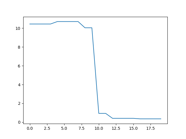
Apply the filter to 1d signal.

>>> signal = np.array([10.0] * 10 + [0.0] * 10)
>>> signal += np.random.random(signal.shape)

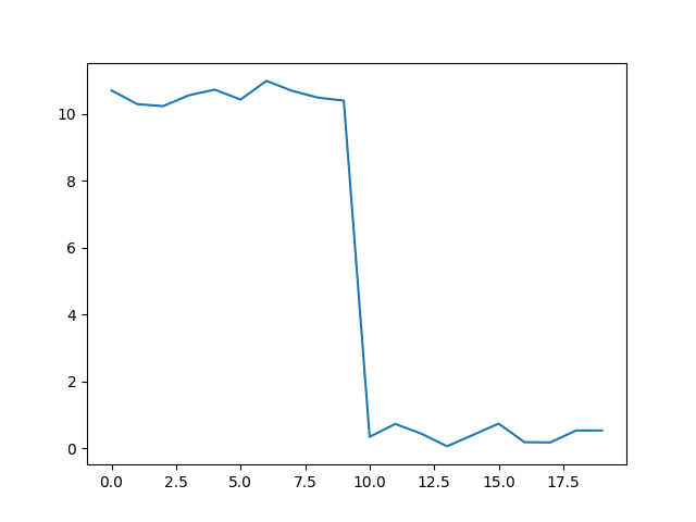
>>> wavelet = "db1"
>>> denoised_signal = wavelet_denoising(signal, wavelet, level=2)

onebone.signal.envelope

Extract envelope.

• Author: Kangwhi Kim

• Contact: kangwhi.kim@onepredict.com

onebone.signal.envelope.envelope_hilbert(x, axis: int = -1) → ndarray

Extract the envelope from the signal using the ‘Hilbert transform’.

Parameters

• x (array_like) – Signal data. Must be real.

• axis (int, default=-1) – Axis along which to do the transformation.

Returns

y (numpy.ndarray) – Envelope of the x, of each 1-D array along axis

onebone.signal.fft

The module about fast fourier transform.

• Author: Daeyeop Na, Kangwhi Kim

• Contact: daeyeop.na@onepredict.com, kangwhi.kim@onepredict.com

onebone.signal.fft.positive_fft(signal: ndarray, fs: Union[int, float], hann: bool = False, normalization: bool = False, axis: int = -1) → Tuple[ndarray, ndarray]

Positive 1D fourier transformation.

Parameters

• signal (numpy.ndarray) – Original time-domain signal

• fs (Union[int, float]) – Sampling rate

• hann (bool, default = False) – hann function used to perform Hann smoothing. It is implemented when hann is True

• normalization (bool, default = False) – Normalization after Fourier transform

• axis (int, default=-1) – The axis of the input data array along which to apply the fourier Transformation.

Returns

• freq (numpy.ndarray) – frequency If input shape is [signal_length,], output shape is freq = [signal_length,]. If input shape is [n, signal_length,], output shape is freq = [signal_length,].

• mag (numpy.ndarray) – magnitude If input shape is [signal_length,], output shape is mag = [signal_length,]. If input shape is [n, signal_length,], output shape is mag = [n, signal_length,].

Examples

>>> n = 400  # array length
>>> fs = 800  # Sampling frequency
>>> t = 1 / fs  # Sample interval time
>>> x = np.linspace(0.0, n * t, n, endpoint=False) # time
>>> y = 3 * np.sin(50.0 * 2.0 * np.pi * x) + 2 * np.sin(80.0 * 2.0 * np.pi * x)
>>> signal = y
>>> freq, mag = positive_fft(signal, fs,  hann = False, normalization = False, axis = -1)
>>> freq = np.around(freq[np.where(mag > 1)])
>>> freq
[50., 80.]

onebone.signal.filter

A frequency filter to leave only a specific frequency band.

and a filter that replaces outlier values in data with other values.

• Author: Kyunghwan Kim, Sunjin Kim

• Contact: kyunghwan.kim@onepredict.com, sunjin.kim@onepredict.com

onebone.signal.filter.bandpass_filter(signal: ndarray, fs: Union[int, float], l_cutoff: Union[int, float], h_cutoff: Union[int, float], order: int = 5, axis: int = -1) → ndarray

1D Butterworth bandpass filter.

Parameters

• signal (numpy.ndarray) – Original time-domain signal.

• fs (Union[int, float]) – Sampling rate.

• l_cutoff (Union[int, float]) – Low cutoff frequency.

• h_cutoff (Union[int, float]) – High cutoff frequency.

• order (int, default=5) – Order of butterworth filter.

• axis (int, default=-1) – The axis of the input data array along which to apply the linear filter.

Returns

out (numpy.ndarray) – Filtered signal. If input shape is [signal_length,], output shape is [signal_length,]. If input shape is [n, signal_length,], output shape is [n, signal_length,].

Examples

Apply the filter to 1d signal. And then check the frequency component of the filtered signal.

>>> fs = 5000.0
>>> t = np.linspace(0, 1, int(fs))
>>> signal = 10.0 * np.sin(2 * np.pi * 20.0 * t)
>>> signal += 5.0 * np.sin(2 * np.pi * 100.0 * t)
>>> signal += 5.0 * np.sin(2 * np.pi * 500.0 * t)
>>> signal.shape
(5000,)
>>> freq_x = np.fft.rfftfreq(signal.size, 1 / fs)[:-1]
>>> origin_fft_mag = abs((np.fft.rfft(signal) / signal.size)[:-1] * 2)
>>> origin_freq = freq_x[np.where(origin_fft_mag > 0.5)]
>>> origin_freq
[ 20., 100., 500.]
>>> filtered_signal = bandpass_filter(signal, fs, l_cutoff=50, h_cutoff=300)
>>> filtered_fft_mag = abs((np.fft.rfft(filtered_signal) / signal.size)[:-1] * 2)
>>> filtered_freq = freq_x[np.where(filtered_fft_mag > 0.5)]
>>> filtered_freq
[ 100.]

Apply the filter to 2d signal (axis=0).

>>> fs = 5000.0
>>> t = np.linspace(0, 1, int(fs))
>>> signal = 10.0 * np.sin(2 * np.pi * 20.0 * t)
>>> signal += 5.0 * np.sin(2 * np.pi * 100.0 * t)
>>> signal = np.stack([signal, signal]).T
>>> signal.shape
(5000, 2)
>>> filtered_signal = bandpass_filter(signal, fs, l_cutoff=50, h_cutoff=300, axis=0)
>>> filtered_fft_mag = abs((np.fft.rfft(filtered_signal[:, 0]) / signal.size)[:-1] * 2)
>>> filtered_freq = freq_x[np.where(filtered_fft_mag > 0.5)]
>>> filtered_freq
[ 100.]

onebone.signal.filter.bandpass_filter_ideal(signal: ndarray, fs: Union[int, float], l_cutoff: Union[int, float], h_cutoff: Union[int, float]) → ndarray

Warning

This method may cause distortion of signal. Generally, this operates well on signals extracted in low resolution. In order to check the distortion of signals, it is recommended to monitor the linear transition of phase.

1D ideal bandpass filter.

Parameters

• signal (numpy.ndarray) – Original time-domain signal.

• fs (Union[int, float]) – Sampling rate.

• l_cutoff (Union[int, float]) – Low cutoff frequency.

• h_cutoff (Union[int, float]) – High cutoff frequency.

Returns

out (numpy.ndarray) – Filtered signal. Input shape is [signal_length,] and output shape is [signal_length,].

Examples

Apply the filter to 1d signal. And then check the frequency component of the filtered signal.

>>> fs = 5000.0
>>> t = np.linspace(0, 1, int(fs))
>>> signal = 10.0 * np.sin(2 * np.pi * 20.0 * t)
>>> signal += 5.0 * np.sin(2 * np.pi * 100.0 * t)
>>> signal += 5.0 * np.sin(2 * np.pi * 500.0 * t)
>>> signal.shape
(5000,)
>>> freq_x = np.fft.rfftfreq(signal.size, 1 / fs)[:-1]
>>> origin_fft_mag = abs((np.fft.rfft(signal) / signal.size)[:-1] * 2)
>>> origin_freq = freq_x[np.where(origin_fft_mag > 0.5)]
>>> origin_freq
[ 20., 100., 500.]
>>> filtered_signal = bandpass_filter_ideal(signal, fs, l_cutoff=50, h_cutoff=300)
>>> filtered_fft_mag = abs((np.fft.rfft(filtered_signal) / signal.size)[:-1] * 2)
>>> filtered_freq = freq_x[np.where(filtered_fft_mag > 0.5)]
>>> filtered_freq
[ 100.]

onebone.signal.filter.bandstop_filter(signal: ndarray, fs: Union[int, float], l_cutoff: Union[int, float], h_cutoff: Union[int, float], order: int = 5, axis: int = -1) → ndarray

1D Butterworth bandstop filter.

Parameters

• signal (numpy.ndarray) – Original time-domain signal.

• fs (Union[int, float]) – Sampling rate.

• l_cutoff (Union[int, float]) – Low cutoff frequency.

• h_cutoff (Union[int, float]) – High cutoff frequency.

• order (int, default=5) – Order of butterworth filter.

• axis (int, default=-1) – The axis of the input data array along which to apply the linear filter.

Returns

out (numpy.ndarray) – Filtered signal. If input shape is [signal_length,], output shape is [signal_length,]. If input shape is [n, signal_length,], output shape is [n, signal_length,].

Examples

Apply the filter to 1d signal. And then check the frequency component of the filtered signal.

>>> fs = 5000.0
>>> t = np.linspace(0, 1, int(fs))
>>> signal = 10.0 * np.sin(2 * np.pi * 20.0 * t)
>>> signal += 5.0 * np.sin(2 * np.pi * 100.0 * t)
>>> signal += 5.0 * np.sin(2 * np.pi * 500.0 * t)
>>> signal.shape
(5000,)
>>> freq_x = np.fft.rfftfreq(signal.size, 1 / fs)[:-1]
>>> origin_fft_mag = abs((np.fft.rfft(signal) / signal.size)[:-1] * 2)
>>> origin_freq = freq_x[np.where(origin_fft_mag > 0.5)]
>>> origin_freq
[ 20., 100., 500.]
>>> filtered_signal = bandstop_filter(signal, fs, l_cutoff=50, h_cutoff=300)
>>> filtered_fft_mag = abs((np.fft.rfft(filtered_signal) / signal.size)[:-1] * 2)
>>> filtered_freq = freq_x[np.where(filtered_fft_mag > 0.5)]
>>> filtered_freq
[ 20., 500.]

Apply the filter to 2d signal (axis=0).

>>> fs = 5000.0
>>> t = np.linspace(0, 1, int(fs))
>>> signal = 10.0 * np.sin(2 * np.pi * 20.0 * t)
>>> signal += 5.0 * np.sin(2 * np.pi * 100.0 * t)
>>> signal = np.stack([signal, signal]).T
>>> signal.shape
(5000, 2)
>>> filtered_signal = bandstop_filter(signal, fs, l_cutoff=50, h_cutoff=300, axis=0)
>>> filtered_fft_mag = abs((np.fft.rfft(filtered_signal[:, 0]) / signal.size)[:-1] * 2)
>>> filtered_freq = freq_x[np.where(filtered_fft_mag > 0.5)]
>>> filtered_freq
[ 20., 500.]

onebone.signal.filter.hampel_filter(x: ndarray, window_size: int, n_sigma: float = 3) → Tuple[ndarray, list]

A hampel filter removes outliers. Estimate the median and standard deviation of each sample using MAD(Median Absolute Deviation) in the window range set by the user. If the MAD > 3 * sigma condition is satisfied, the value is replaced with the median value.

\[m_i = median(x_{i-k_{left}}, x_{i-k_{left}+1}, ..., x_{i+k_{right}-1}, x_{i+k_{right}})\]

\[MAD_i = median(|x_{i-k}-m_{i}|,...,|x_{i+k}-m_{i}|)\]

\[{\sigma}_i = {\kappa} * MAD_i\]

Where \(k_{left}\) and \(k_{right}\) are the number of neighbors on the left and right sides, respectively, based on x_i (\(k_{left} + k_{right}\) = window samples). \(m_i\) is Local median, \(MAD_i\) is median absolute deviation which is the residuals (deviations) from the data’s median. \({\sigma}_i\) is the MAD may be used similarly to how one would use the deviation for the average. In order to use the MAD as a consistent estimator for the estimation of the standard deviation \({\sigma}\), one takes \({\kappa} * MAD_i\). \({\kappa}\) is a constant scale factor, which depends on the distribution. For normally distributed data \({\kappa}\) is taken to be \({\kappa}\) = 1.4826

Parameters

• x (numpy.ndarray) – 1d-timeseries data. The shape of x must be (signal_length,) .

• window_size (int) – Lenght of the sliding window. Only integer types are available, and the window size must be adjusted according to your data.

• n_sigma (float, defalut=3) – Coefficient of standard deviation.

Returns

• filtered_x (numpy.ndarray) – A value from which outlier or NaN has been removed by the filter.

• index (list) – Returns the index corresponding to outlier.

References

[1] Pearson, Ronald K., et al. “Generalized hampel filters.” EURASIP Journal on Advances in Signal Processing 2016.1 (2016): 1-18. DOI: 10.1186/s13634-016-0383-6

Examples

>>> fs = 1000.0
>>> t = np.linspace(0, 1, int(fs))
>>> y = np.sin(2 * np.pi * 10.0 * t)
>>> np.put(y, [13, 124, 330, 445, 651, 775, 978], 3)
>>> plt.plot(y) # noise_signal

>>> filtered_signal = hampel_filter.hampel_filter(y, window_size=5)[0]
>>> plt.plot(filtered_signal) # filtered_signal

onebone.signal.filter.highpass_filter(signal: ndarray, fs: Union[int, float], cutoff: Union[int, float], order: int = 5, axis: int = -1) → ndarray

1D Butterworth highpass filter.

Parameters

• signal (numpy.ndarray) – Original time-domain signal.

• fs (Union[int, float]) – Sampling rate.

• cutoff (Union[int, float]) – Cutoff frequency.

• order (int, default=5) – Order of butterworth filter.

• axis (int, default=-1) – The axis of the input data array along which to apply the linear filter.

Returns

out (numpy.ndarray) – Filtered signal.

Examples

Apply the filter to 1d signal. And then check the frequency component of the filtered signal.

>>> fs = 5000.0
>>> t = np.linspace(0, 1, int(fs))
>>> signal = 10.0 * np.sin(2 * np.pi * 20.0 * t)
>>> signal += 5.0 * np.sin(2 * np.pi * 100.0 * t)
>>> signal.shape
(5000,)
>>> freq_x = np.fft.rfftfreq(signal.size, 1 / fs)[:-1]
>>> origin_fft_mag = abs((np.fft.rfft(signal) / signal.size)[:-1] * 2)
>>> origin_freq = freq_x[np.where(origin_fft_mag > 0.5)]
>>> origin_freq
[ 20., 100.]
>>> filtered_signal = highpass_filter(signal, fs, cutoff=50)
>>> filtered_fft_mag = abs((np.fft.rfft(filtered_signal) / signal.size)[:-1] * 2)
>>> filtered_freq = freq_x[np.where(filtered_fft_mag > 0.5)]
>>> filtered_freq
[ 100.]

Apply the filter to 2d signal (axis=0).

>>> fs = 5000.0
>>> t = np.linspace(0, 1, int(fs))
>>> signal = 10.0 * np.sin(2 * np.pi * 20.0 * t)
>>> signal += 5.0 * np.sin(2 * np.pi * 100.0 * t)
>>> signal = np.stack([signal, signal]).T
>>> signal.shape
(5000, 2)
>>> filtered_signal = highpass_filter(signal, fs, cutoff=50, axis=0)
>>> filtered_fft_mag = abs((np.fft.rfft(filtered_signal[:, 0]) / signal.size)[:-1] * 2)
>>> filtered_freq = freq_x[np.where(filtered_fft_mag > 0.5)]
>>> filtered_freq
[ 100.]

onebone.signal.filter.lowpass_filter(signal: ndarray, fs: Union[int, float], cutoff: Union[int, float], order: int = 5, axis: int = -1) → ndarray

1D Butterworth lowpass filter.

Parameters

• signal (numpy.ndarray) – Original time-domain signal.

• fs (Union[int, float]) – Sampling rate.

• cutoff (Union[int, float]) – Cutoff frequency.

• order (int, default=5) – Order of butterworth filter.

• axis (int, default=-1) – The axis of the input data array along which to apply the linear filter.

Returns

out (numpy.ndarray) – Filtered signal.

Examples

Apply the filter to 1d signal. And then check the frequency component of the filtered signal.

>>> fs = 5000.0
>>> t = np.linspace(0, 1, int(fs))
>>> signal = 10.0 * np.sin(2 * np.pi * 20.0 * t)
>>> signal += 5.0 * np.sin(2 * np.pi * 100.0 * t)
>>> signal.shape
(5000,)
>>> freq_x = np.fft.rfftfreq(signal.size, 1 / fs)[:-1]
>>> origin_fft_mag = abs((np.fft.rfft(signal) / signal.size)[:-1] * 2)
>>> origin_freq = freq_x[np.where(origin_fft_mag > 0.5)]
>>> origin_freq
[ 20., 100.]
>>> filtered_signal = lowpass_filter(signal, fs, cutoff=50)
>>> filtered_fft_mag = abs((np.fft.rfft(filtered_signal) / signal.size)[:-1] * 2)
>>> filtered_freq = freq_x[np.where(filtered_fft_mag > 0.5)]
>>> filtered_freq
[ 20.]

Apply the filter to 2d signal (axis=0).

>>> fs = 5000.0
>>> t = np.linspace(0, 1, int(fs))
>>> signal = 10.0 * np.sin(2 * np.pi * 20.0 * t)
>>> signal += 5.0 * np.sin(2 * np.pi * 100.0 * t)
>>> signal = np.stack([signal, signal]).T
>>> signal.shape
(5000, 2)
>>> filtered_signal = lowpass_filter(signal, fs, cutoff=50, axis=0)
>>> filtered_fft_mag = abs((np.fft.rfft(filtered_signal[:, 0]) / signal.size)[:-1] * 2)
>>> filtered_freq = freq_x[np.where(filtered_fft_mag > 0.5)]
>>> filtered_freq
[ 20.]

onebone.signal.smoothing

A Moving Average (MA) which returns the weighted average of array.

• Author: Kibum Park

• Contact: kibum.park@onepredict.com

onebone.signal.smoothing.moving_average(signal: ndarray, window_size: Union[int, float], pad: bool = False, weights: Optional[ndarray] = None, axis: Union[int, float] = -1) → ndarray

Weighted moving average. .. math:: WMA(x, w, t, n) = sum_{i=n-t+1}^{n} w_i x_i, where \(x\) is the input array, \(w_i\) is the weight of the \(i\)-th element, \(t\) is the window size, \(n\) is the \(n\) is smaller than \(t\), \(i\) is set to \(0\).

Parameters

• signal (numpy.ndarray of shape (signal_length,), (n, signal_length,)) – Original time-domain signal.

• window_size (Union[int, float], optional, default=10) – Window size. One of window_size,`weights` must be specified.

• pad (bool, default=False) – Padding method. If True, Pads with the edge values of array is added. So the shape of output is same as signal.

• weights (Union[numpy.ndarray of shape (window_size,), None], optional, default=None) – Weighting coefficients. If None, the weights are uniform. One of window_size,`weights` must be specified.

• axis (Union[int, float], optional, default=-1) – The axis of the input data array along which to apply the moving average.

Returns

ma (numpy.ndarray) – Moving average signal. If input shape is [signal_length,], output shape is [signal_length,]. If input shape is [n, signal_length,] and axis is 1, output shape is [n, signal_length,]. If input shape is [signal_length, n] and axis is 0, output shape is [signal_length, n]. If pad is False, output shape is [signal_length - window_size + 1,]. If pad is True, output shape is [signal_length,].

Examples

>>> signal = np.array([1, 2, 3, 4, 5, 6, 7, 8, 9, 10])
>>> window_size = 3
>>> moving_average(signal, window_size)
[2, 3, 4, 5, 6, 7, 8, 9]

>>> signal = np.array([1, 2, 3, 4, 5, 6, 7, 8, 9, 10])
>>> window_size = 3
>>> moving_average(signal, window_size, pad=True)
[1, 1.5, 2, 3, 4, 5, 6, 7, 8, 9]

>>> signal = np.array([1, 2, 3, 4, 5, 6, 7, 8, 9, 10])
>>> window_size = 3
>>> weights = np.array([1, 2, 3])
>>> moving_average(signal, window_size, weights=weights)
[2.33333333, 3.33333333, 4.33333333, 5.33333333, 6.33333333, 7.33333333, 8.33333333, 9.33333333]